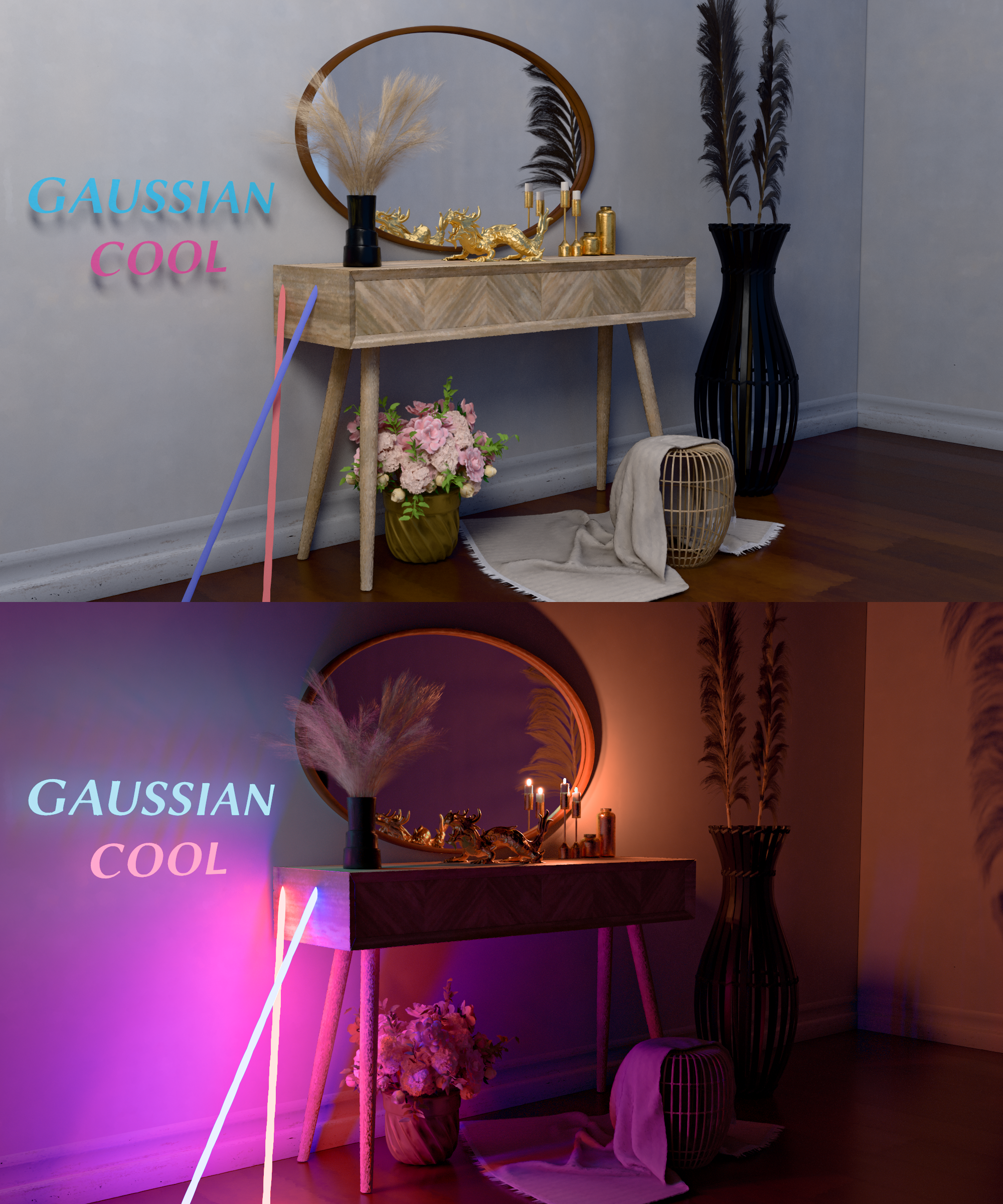
TL;DR

• Path tracing a scene made of 3D Gaussian primitives with arbitrary illumination.
• Volumetric formulation but with a focus to accommodate opaque geometries.
• Flexible appearance supporting glossy and diffuse objects (and more).
• Versatile forward rendering and differentiable rendering applications.

Motivation

3D Gaussians are powerful to represent complex geometries, but so far, most applications like 3D Gaussian Splatting (3DGS) only use them for radiance fields. In fact, we felt it was a shame to limit Gaussians to radiance fields. Can we use Gaussians to build a scene for general-purpose rendering with different lighting conditions, just like how we use triangles? This paper enables exact this. We will talk about how to use Gaussians in a meaningful way such that we can run path tracing on them to properly simulate global illumination.

What is a Gaussian primitive?

We want a Gaussian to be a “basic unit” of our scene representation. In 3DGS, it suffices to associate a opacity and a color (or a set of sperical harmonics coefficients) with each Gaussian. However, we need more to define Gaussians for light transport. It boils down to two parts, a transmittance function (or equivalently, a free-flight distirbution) and a phase function. These should be familiar concepts to those who have experience with volumetric light transport. The transmittance function determines how likely light will be scattered, and the phase function determines the appearance. With these two pieces of information, a Gaussian primitive behaves just like a triangle but in a probabilistic way.

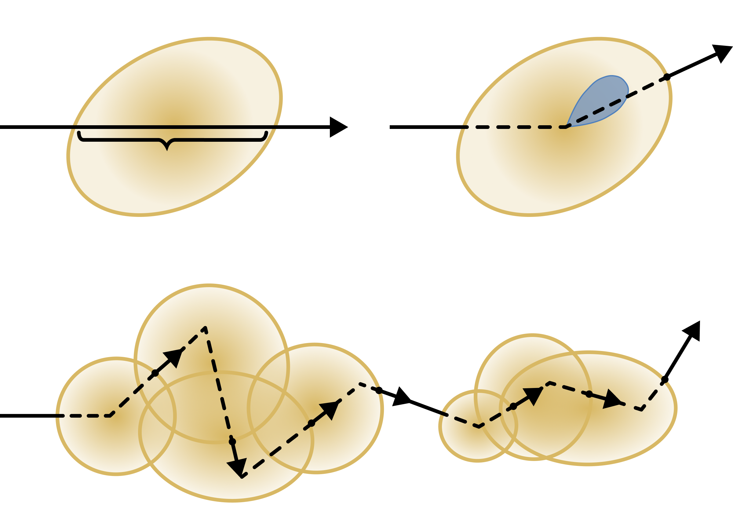
Transmittance function (free-flight PDF)

The volumetric formulation gives us a continuous representation that supports transparency and partial occlusion. At the same time, we don’t necessarily want to limit ourselves to traditional participating media such as clouds and smoke. In fact, we do want to accommodate objects made of opaque. Therefore, we use linear transmittance for our Guassian primitive, which is a type of non-exponential transmittance functions shown to adapt to opaque surfaces better. Let \( G_k(x) \) be one 3D Gaussian distribution, the free-flight PDF is simply

We can get the transmittance by 1 minus integrating over the free-flight PDF:

The max operator at the end clamp the transmittance value to the valid range between 0 and 1. This corresponds to a maximum distance at which the light is guaranteed to be blocked \( t_{\mathrm{sat}} \) (could be infinity), which we call the saturating distance.

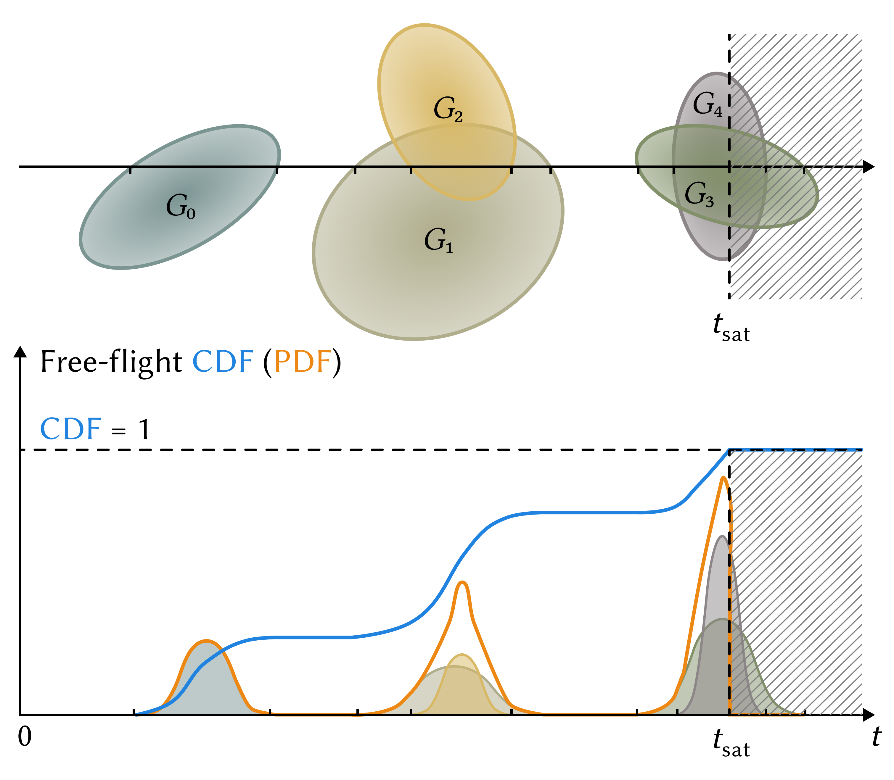
In the paper, we provide an efficient sampling algorithm to sample the free-flight PDF in a heterogeneous scene to enable Monte Carlo path tracing.

Phase function

Unlike a triangle, there is not always a singular “surface normal” for a Gaussian primitive. A Gaussian primitive can represent a simple surface patch or a collection of small surface elements with different orientations. Therefore, a useful appearance model for the primitive should incorporate this aggregated effect while still being compatible with simple flat scenarios. Our goal here is to have a flexible phase function so that we can incorporate different geometric configurations and reflectance properties. We define the phase function to be an inner product of an SGGX visible NDF function, \( D_{\omega_o}(n) \), and a base surface BSDF, \( f(\omega_i, \omega_o) \):

In the example below from left to right, we show a more surface-like configuration, an isotropic configuration, and a fiber-like configuration where we have some interesting sheen effect emerging from the NDF.

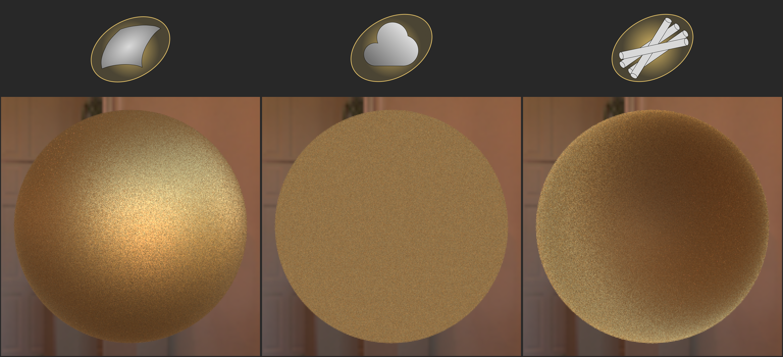
In the paper, we describe how to evaluate and importance sample the phase function so that our Gaussian primitive can be integrated seamlessly into a Monte Carlo renderer.

Results

We demonstrate the versatility of our Gaussian primitive to represent objects with a wide range of geometric and material characteristics. Our framework supports full, unbiased global illumination with Monte Carlo (volumetric) path tracing, capable of producing and not limited to effects such as soft shadow, glossy reflection, interreflection. See teaser and the supplemental videos for examples.

We can render scenes acquired from existing data in different formats, such as meshes or 3DGS-initialized scenes. The conversion process, including gradient-based transmittance refinement, is described in the paper.

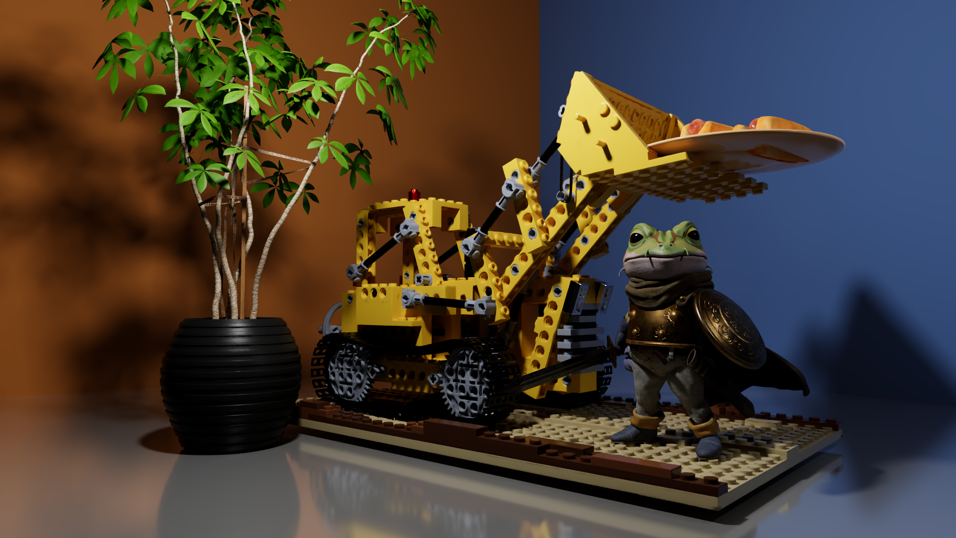
Here is a render using the NeRF Blender synthetic dataset and this fantastic Sir Frog model from Chrono Trigger:

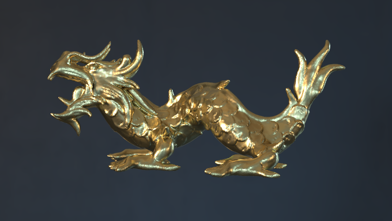
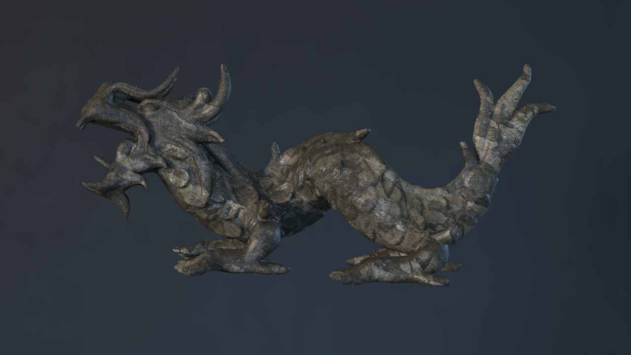
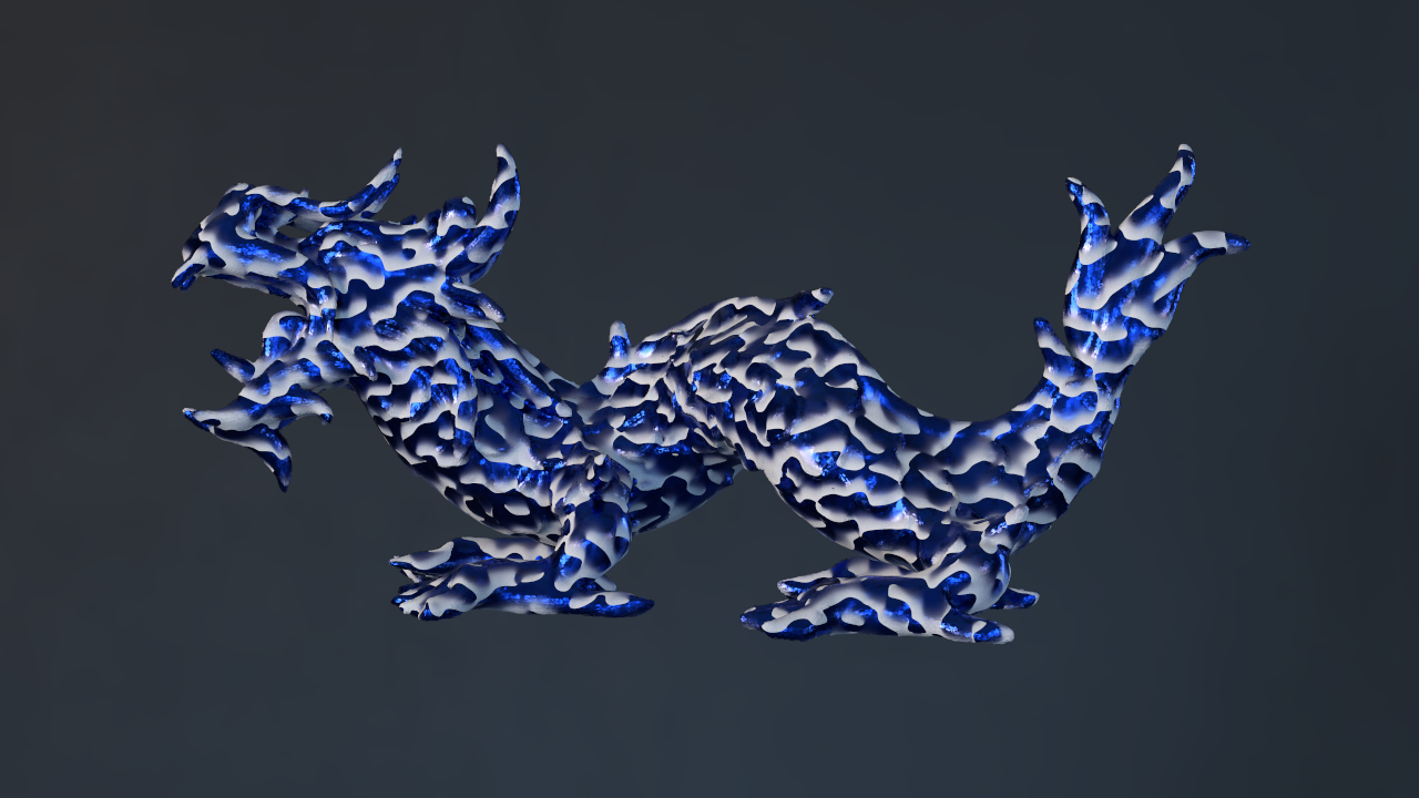
Here is another example with different materials applied:

Original	New material 1	New material 2

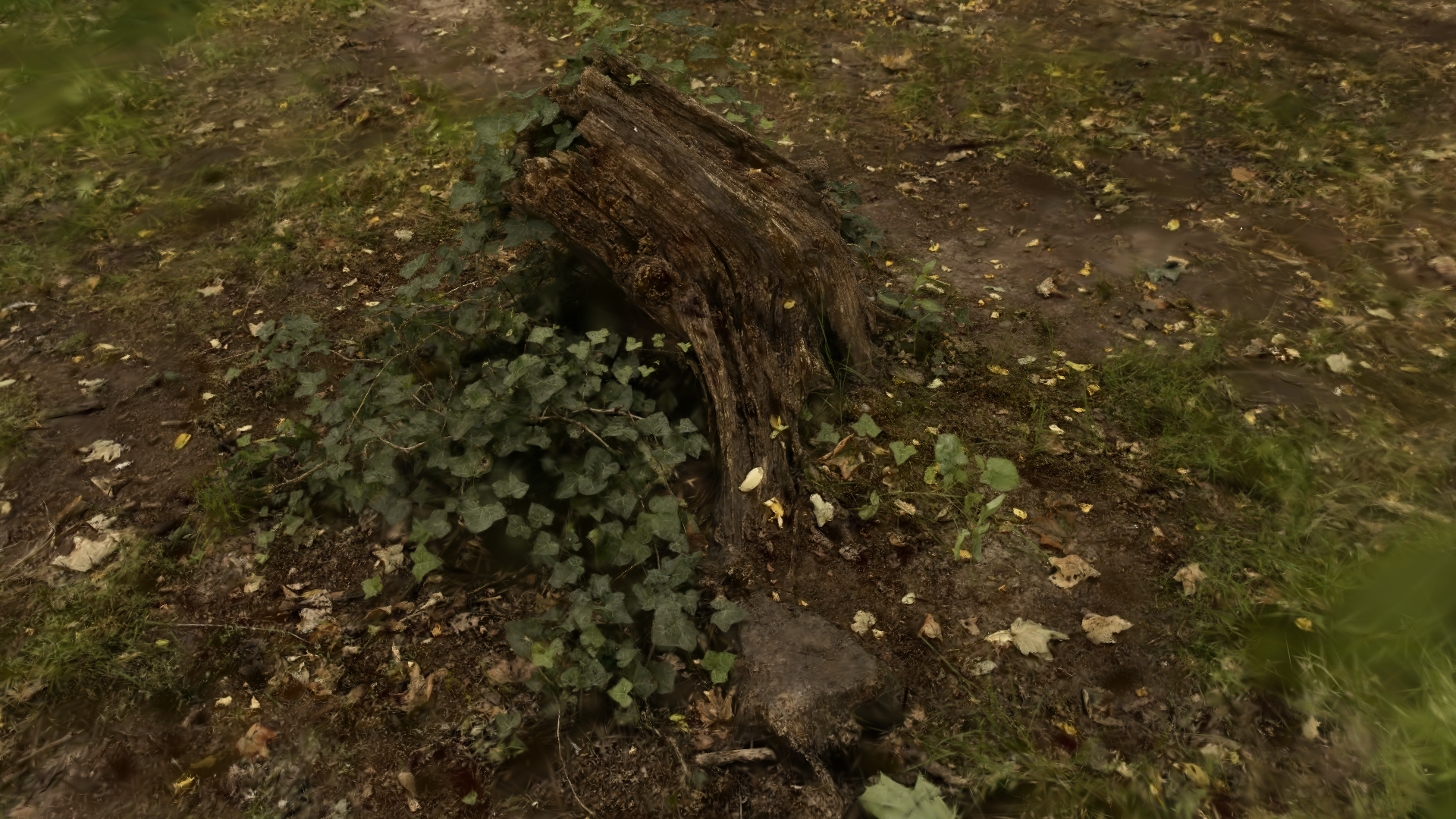
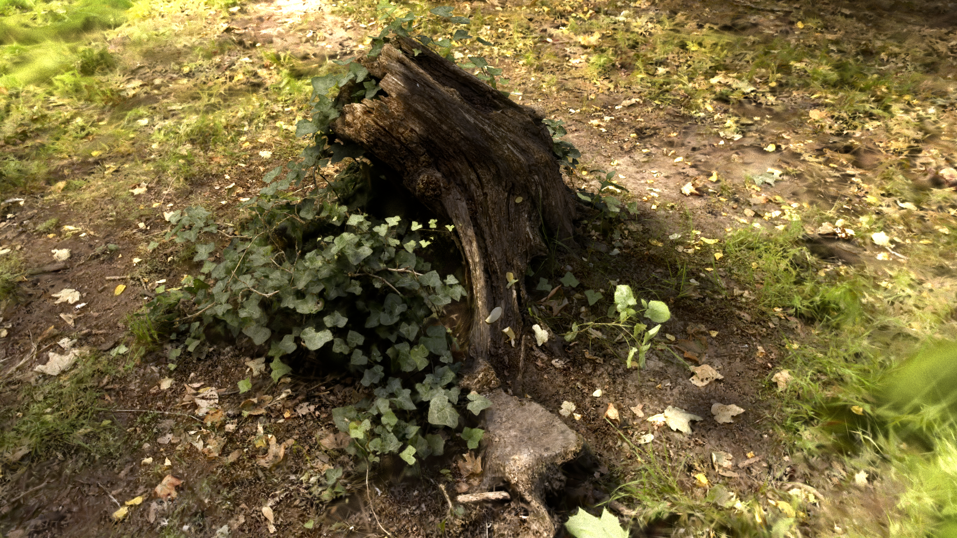
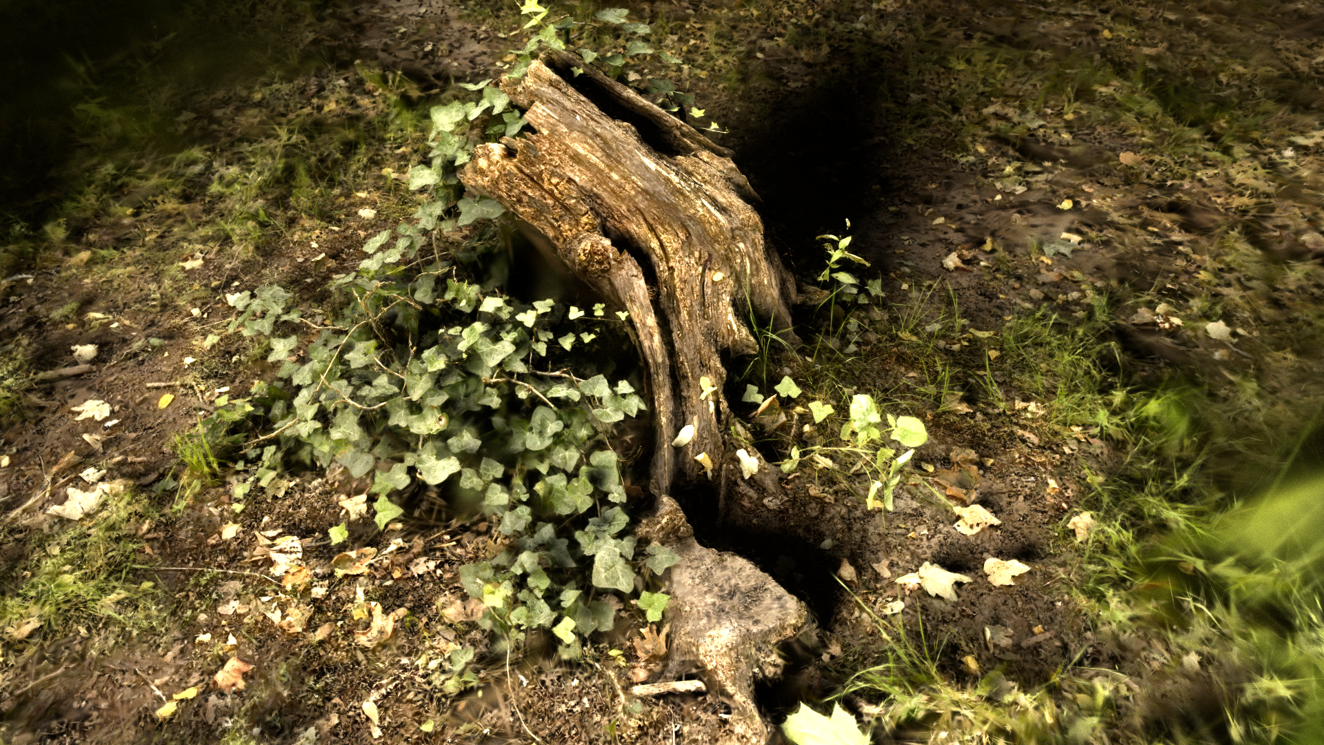
This also gives us the ability to (empirically) re-render real-world scenes under new lighting conditions:

Original	New lighting 1	New lighting 2

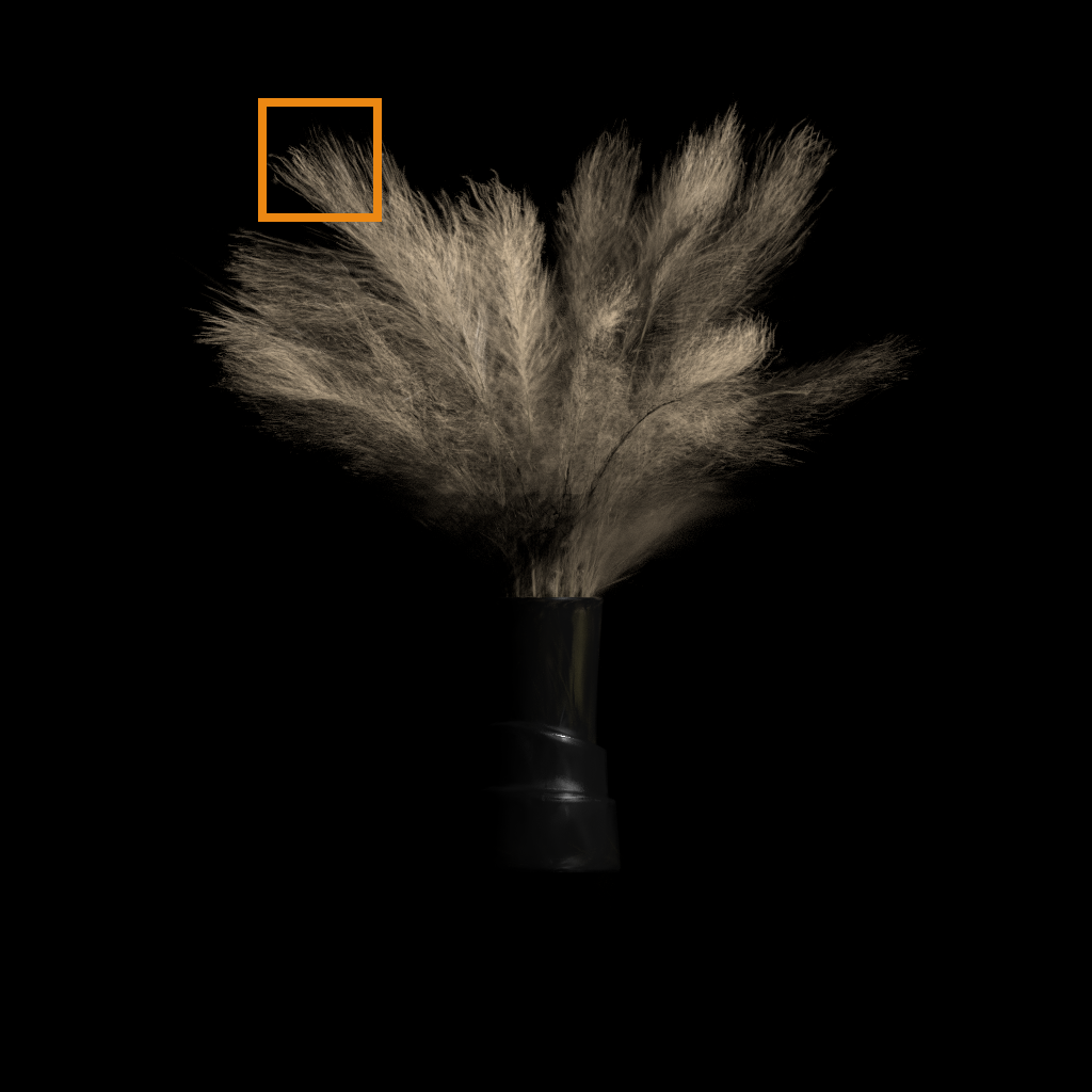
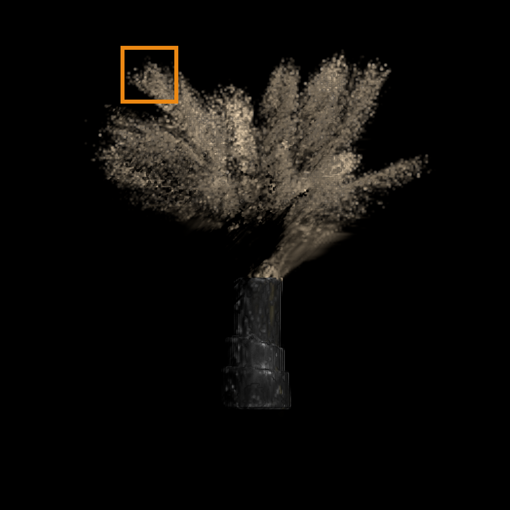
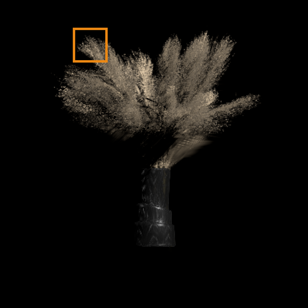
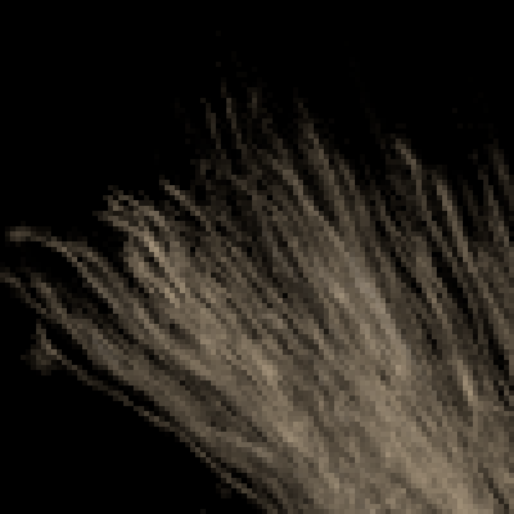
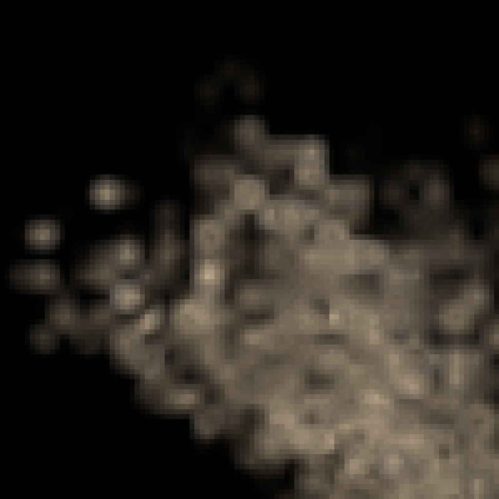
We also extensively discuss when and how our representation can be beneficial over other surface/volumetric representations. For example, it is more efficient to capture high-frequency details than voxels.

Ours	Voxels (Eq. num)	Voxels (8x)

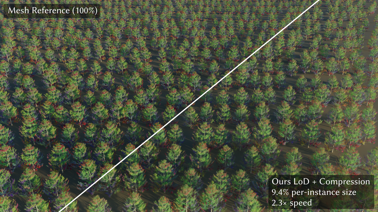
On the other hand, compared to meshes, our representation also excels at representing aggregated elements such as foliage. With a basic discrete LoD scheme and codebook-based compression, we can achieve significant memory reduction and speedup over the mesh baseline with minimal perceptual difference.

Among other applications, we also show that our formulation is “backward-compatible” with radiance field reconstruction since radiance fields are essentially a special case of the general volumetric light transport. Check out the paper for many more results and comparisons.

Video

BibTeX

@article{zhou2026unified,
      title={Unified Gaussian Primitives for Scene Representation and Rendering}, 
      author={Yang Zhou and Songyin Wu and Lingqi Yan},
      year={2026},
      note = {Just Accepted},
      journal = {ACM Trans. Graph.},
      month = jun,
}